How to use Wannier90 Apptainer image

For more information on Apptainer containers and their use, we provide a description of Apptainer, a crash course on how to use Apptainer, and of course there’s also the official Apptainer’s documentation.

Input files

To illustrate the various commands, a set of Wannier90 input files is available in the form of an archive via this link.

Those files correspond to the first two tutorials of the Wannier90 official documentation. Wannier90 is a post-processing tool: it only reads files previously generated by a first-principles electronic structure code and does not perform any DFT calculation. The archive contains two directories, one per tutorial.

tuto1: tutorial 1 (Gallium Arsenide — MLWFs for the valence bands), with the original input files and a worked solution. It contains:

• gaas.win: the master input file. It defines the crystal structure of gallium arsenide (GaAs), the number of Wannier functions to compute (4), the k-point grid (2×2×2), and the starting guess for the Wannier functions.
• gaas.mmn: the overlap matrices $M^{(\mathbf{k},\mathbf{b})}$ between the periodic parts of the Bloch states at neighboring k-points.
• gaas.amn: the projections $A^{(\mathbf{k})}$ of the Bloch states onto a set of trial localized orbitals.
• UNK00001.1 to UNK00008.1: the Bloch states in the real-space unit cell, one file per k-point (8 files). They are only needed to plot the Wannier functions.

tuto2: tutorial 2 (Lead — Wannier-interpolated Fermi surface), with the original input files and a worked solution. It contains:

• lead.win: the master input file. It defines the crystal structure of lead (one Pb atom in the face-centered cubic primitive cell), the number of Wannier functions to compute (4), the k-point grid (4×4×4), the starting guess for the Wannier functions, and the keywords for the Fermi surface calculation.
• lead.mmn: the overlap matrices $M^{(\mathbf{k},\mathbf{b})}$.
• lead.amn: the projections $A^{(\mathbf{k})}$ of the Bloch states onto a set of trial localized orbitals.
• lead.eig: the Bloch eigenvalues at each k-point. They are only needed for the band interpolation.

In this tutorial, we will assume that the archive is extracted in the current directory. To extract it:

tar -xzf wannier90-tutorial-inputs.tar.gz

Quickstart

For impatient folks, here is how to launch the Wannier90 computations using the container image in the case where the current directory contains the wannier90.sif container image and the extracted tuto1 and tuto2 directories:

cd tuto1
apptainer exec ../wannier90.sif wannier90.x gaas
cd ../tuto2
apptainer exec ../wannier90.sif wannier90.x lead

Detailed usage for the Wannier90 container

This section explains how to use the Wannier90 image. For more details about Apptainer commands, please look at this tutorial.

Introduction

Wannier90 is an open-source code for computing maximally-localized Wannier functions (MLWFs) in condensed matter physics. It is used as a post-processing tool for first-principles electronic structure codes such as Quantum ESPRESSO, VASP or Abinit, and is applied to band-structure interpolation and to the calculation of electronic properties of metals, insulators and topological materials.

The main executable in the image is the wannier90.x executable. The following command displays the version of the executable:

apptainer exec wannier90.sif wannier90.x --version

The code license can be accessed from outside the container as follows:

w_path=$(apptainer exec wannier90.sif ls /gnu/store | grep wannier)
license=$(apptainer exec wannier90.sif find /gnu/store/$w_path -name "LICENSE")
apptainer exec wannier90.sif cat $license

Tutorial 1: MLWFs for the valence bands of GaAs, with plotting

Description of the example

The input files provided in this tutorial are extracted from the Wannier90 official tutorial 1 (Gallium Arsenide — MLWFs for the valence bands). The example computes the four MLWFs spanning the four valence bands of GaAs, and then plots them on a real-space grid. The main input file, gaas.win, defines the system and job parameters, including:

• Wannier functions: num_wann = 4 Wannier functions, optimized for at most num_iter = 20 iterations.
• Unit cell and atoms: the face-centered cubic primitive cell (given in Bohr).
• Starting guess: As:sp3 projections, i.e. four sp³-like orbitals centred on As. The official tutorial describes this starting guess as four bond-centred Gaussians.
• K-points: a 2×2×2 Monkhorst-Pack grid (mp_grid) and the list of the 8 k-points.
• Wavefunction format: wvfn_formatted=.true. reads the Bloch states (UNK files) from formatted text files, which ensures the example works on all platforms. The default (unformatted) should be used in production runs.
• Plotting: wannier_plot = true asks Wannier90 to write the MLWFs on a real-space grid, in addition to minimizing their spread.

The first run of the official tutorial is done without the wannier_plot keyword, in order to only minimize the spread. The plotting step is slower and uses more memory, because the MLWFs must then be represented explicitly on a real-space grid. The gaas.win file of this tutorial directly includes wannier_plot = true.

Running the simulation

The following commands run Wannier90 on the gaas seed name. All input files share this prefix, and the output files are written in the current directory with the same prefix.

cd tuto1
apptainer exec ../wannier90.sif wannier90.x gaas

Reading the results

After the job completes, the following output files are generated:

• gaas.wout: main output file, containing the k-point mesh analysis, the spread minimization and the plotting summary.
• gaas.chk: checkpoint file.
• gaas_00001.xsf to gaas_00004.xsf: the four MLWFs on a real-space grid, in XCrySDen format.

The MLWFs written in the .xsf files can be visualized with XCrySDen. For example, we can use the XCrySDen container image provided by the platform:

apptainer exec ../xcrysden.sif xcrysden --xsf gaas_00001.xsf

Once XCrySDen starts, the following settings can be set in Tools → Data Grid to visualize the results:

Degree of triCubic Spline = 3;
Isovalue = 0.95;
Render +/- isovalue = yes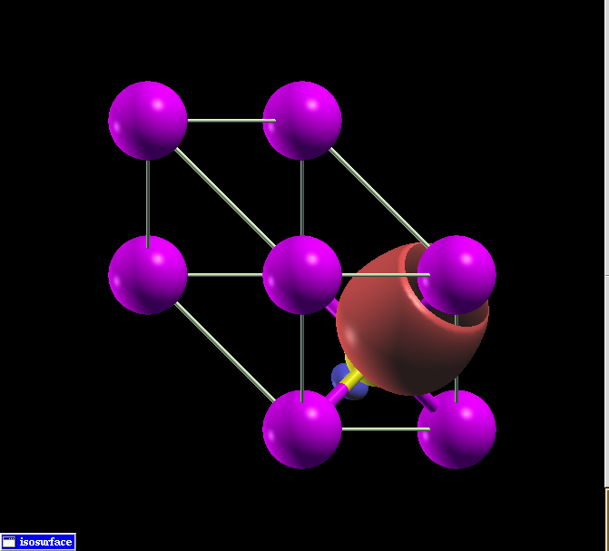

Tutorial 2: Wannier-interpolated Fermi surface of lead

Description of the example

The input files provided in this tutorial are extracted from the Wannier90 official tutorial 2 (Lead — Wannier-interpolated Fermi surface). The example computes the MLWFs for the four lowest states of lead, and then uses Wannier interpolation to plot its Fermi surface. The four lowest valence bands of lead are separated in energy from the higher conduction states, but the MLWFs of these states are partially occupied: MLWFs describing only the occupied states would be poorly localized. The main input file, lead.win, defines the system and job parameters, including:

• Wannier functions: num_wann = 4 Wannier functions, optimized for at most num_iter = 20 iterations.
• Unit cell and atoms: the face-centered cubic primitive cell (given in Bohr) with one Pb atom at the origin.
• Starting guess: Pb:sp3 projections, i.e. atom-centered sp³ hybrid orbitals.
• K-points: a 4×4×4 Monkhorst-Pack grid (mp_grid) and the list of the 64 k-points.
• Fermi surface: fermi_surface_plot = true asks Wannier90 to compute the Fermi surface, and fermi_energy = 5.2676 sets the Fermi energy (in eV), which was obtained from the initial first-principles calculation.

In the official tutorial, the spread of the MLWFs is first minimized in a run without the Fermi surface keywords. The unitary transformations obtained are then reused, by adding restart = plot to the input file, to interpolate the band energies on a dense mesh of k-points without repeating the whole calculation. The lead.win file of this tutorial has already been modified so that both operations are done in a single run, without any restart.

Running the simulation

The following command runs Wannier90 on the lead seed name:

cd tuto2
apptainer exec ../wannier90.sif wannier90.x lead

Reading the results

After the job completes, the following output files are generated:

• lead.wout: main output file, containing the k-point mesh analysis, the spread minimization and the plotting summary.
• lead.chk: checkpoint file.
• lead.bxsf: the Wannier-interpolated Fermi surface, in XCrySDen format.

The lead.bxsf file contains the energies of the four bands at the Fermi energy of $5.2676~eV$, on a 51×51×51 grid of the reciprocal unit cell. The density of the grid is controlled by the fermi_surface_num_points keyword, whose default value is 50 (i.e. 50³ points).

The Fermi surface can be visualized with XCrySDen. For example, we can use the XCrySDen container image provided by the platform:

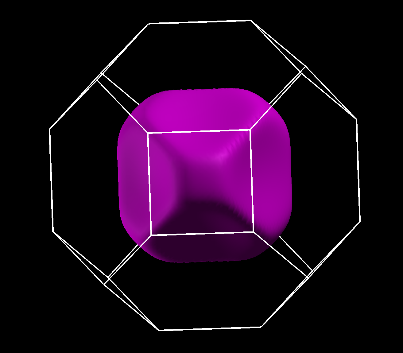
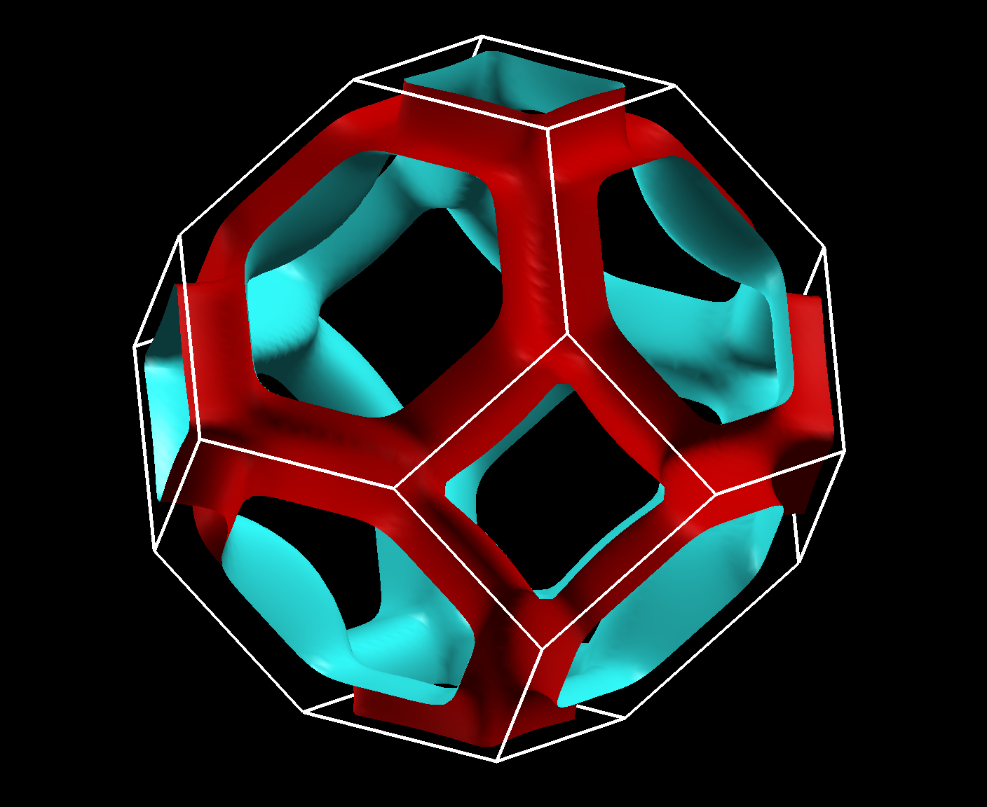
apptainer exec ../xcrysden.sif xcrysden --bxsf lead.bxsf

The following screenshots show the Wannier-interpolated Fermi surface of lead for band 1 and band 3 respectively, as displayed by XCrySDen.