Input files

To illustrate the various commands, a RASPA2 input file is available in the form of an archive via this link. This file is named MC_methane.input and corresponds to a tutorial example from the RASPA2 manual.

In this tutorial, we will assume that the input file contained in this archive is in the current directory. To extract it:

tar -xzf raspa2-tutorial-inputs.tar.gz

Quickstart

For impatient folks, here is how to launch a RASPA2 computation in the case where the current directory contains the raspa2.sif container image and the MC_methane.input input file:

apptainer exec raspa2.sif simulate -i MC_methane.input -d /

Detailed usage for the RASPA2 container

This section explains how to use the RASPA2 image. For more details about Apptainer commands, please look at this tutorial.

Introduction

RASPA2 is an advanced software package designed for the simulation of adsorption and diffusion in porous materials. It employs Monte Carlo and molecular dynamics methods to explore thermodynamic and transport properties under various conditions.

The main executable in the image is the simulate executable. The software version can be displayed with the following command:

apptainer exec raspa2.sif simulate -v

The code license can be accessed from outside the container as follows:

raspa_path=$(apptainer exec raspa2.sif ls /gnu/store | grep raspa)
apptainer exec raspa2.sif cat /gnu/store/$raspa_path/share/doc/raspa2-2.0.48/LICENSE

The input file MC_methane.input corresponds to the first basic example of the RASPA2 manual titled Example 1: Monte Carlo of methane in a box, presented as:

A Monte Carlo run of 100 methane molecules in a 30 × 30 × 30 Å box.

The input file has been extracted from the software repository, under examples/Basic/1_MC_Methane_in_Box/simulation.input.

Running the simulation

The following command runs the simulation using the RASPA2 container image and may take a few seconds to complete:

apptainer exec raspa2.sif simulate -i MC_methane.input -d /

In order to run the previous simulation, the software needs to have access to some additional files, namely:

• pseudo_atoms.def: contains pseudo-potentials for various atomic and molecular species,
• force_field_mixing_rules.def: defines interaction parameters and mixing rules for the force field,
• methane.def: defines the molecular properties of methane.

Those files are stored in the container image, under the /share/raspa/forcefield/ExampleMoleculeForceField path for the first two files and under the /share/raspa/molecules/ExampleDefinitions for the last one. As a generalizable example, the following command copies methane.def in the current directory:

apptainer exec raspa2.sif cp /share/raspa/forcefield/ExampleMoleculeForceField/methane.def ./

The -d option in the simulate command is used to set the path to the RASPA2 directory containing the previous files. The software then automatically looks for the needed files in /share/raspa. When this option is not provided, the software looks for the needed files in the current directory. This can be useful when working with custom pseudo-potentials, force fields or molecule properties.

The simulation produces four different folders: Movies, Output, Restart and VTK.

Visualizing the simulation movies with VMD software

VMD software can be used to visualize the movies produced by the simulation. The VMD container image of the DIAMOND project can be used for this purpose.

The following command opens the visualization software graphical user interface (GUI):

apptainer exec vmd.sif vmd

The .pdb movies in the Movies/System_0 directory can be opened from the GUI with the File/New molecule/Browse button, then loaded with the Load button. The names of the files embed the external temperature (here $300~K$) as well as the pressure ($0~Pa$ here) set by the simulation.

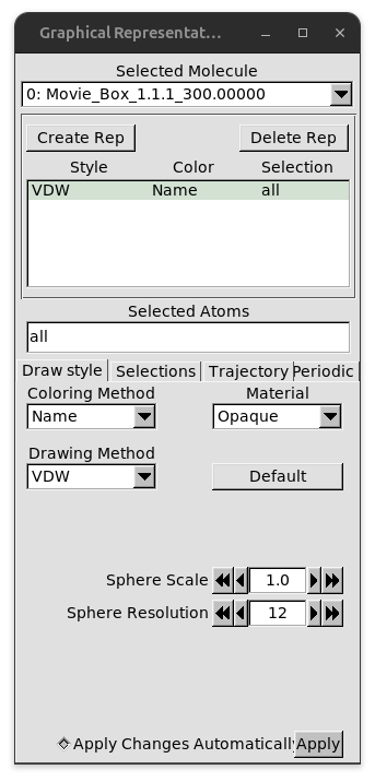
Once the chosen file is loaded in VMD GUI, a simple representation can be created from the Graphics/Representations menu by selecting VDW for the Drawing Method and Name for the Coloring Method, as shown below.

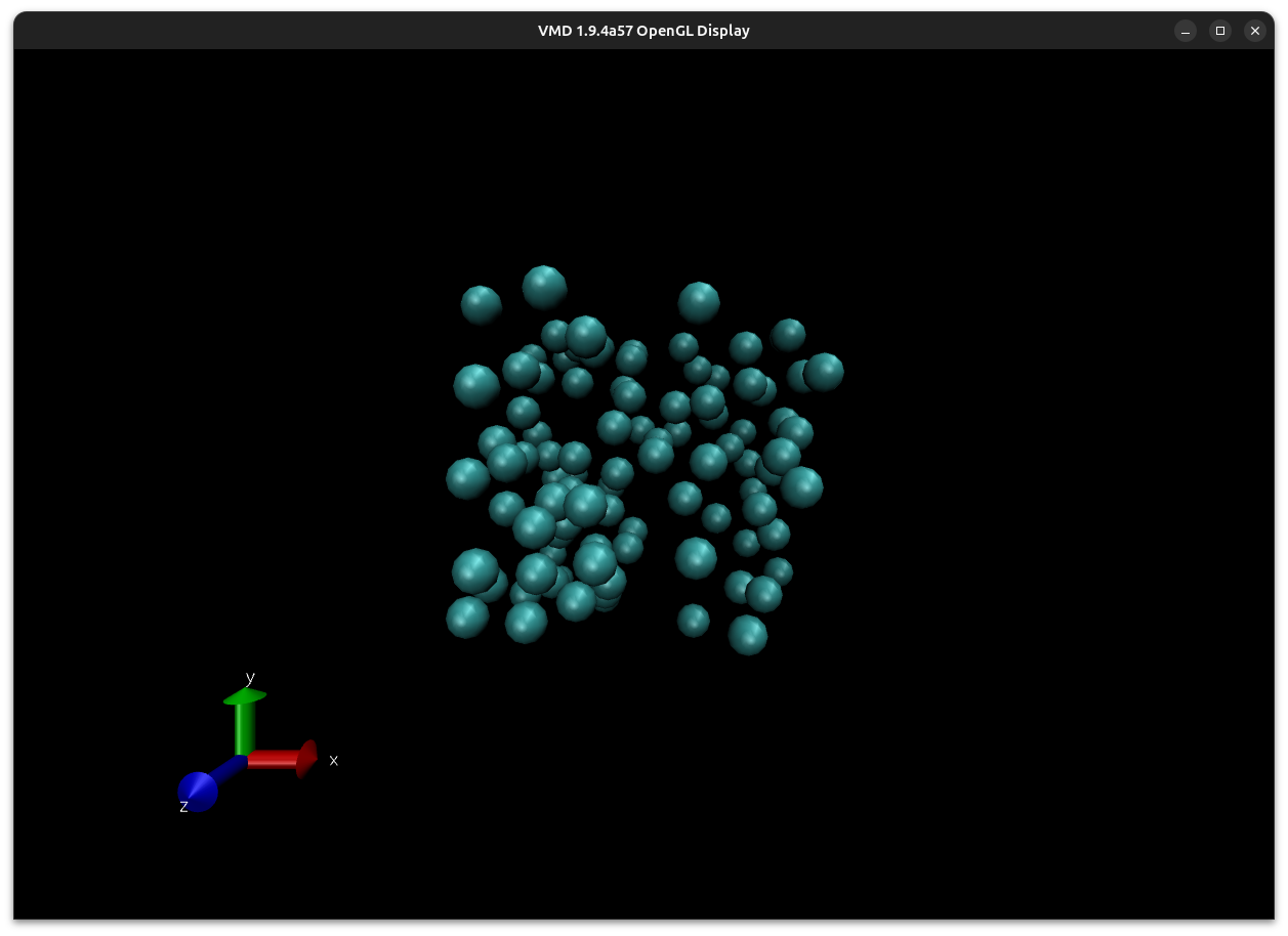
Once applied, the movie can be run with the black arrow button in the lower-right corner of VMD main interface. As an example, the following screenshot shows a frame from the Movie_Box_1.1.1_300.000000_0.000000_allcomponents.pdb movie.

Analyzing simulation results

The output of the simulation is written in the Output/System_0/output_Box_1.1.1_300.000000_0.data text file. One key information contained in this file is the energy-drift status:

Total energy-drift: -7.21955e-11

According to the manual:

In Monte Carlo, only differences in energies are computed. These differences are continuously added to keep track of the current energies (from which average energies etc. are computed). Obviously, the current energy that is kept track off during the simulation should be equal to a full recalculation of the energies. The difference between the two signals an error. If the drift is higher than say 1e − 3 or 1e − 4 the results of the simulation are in error. This could be due to an error in one of the Monte Carlo moves or because the force field is “wrong” (a typical error is when one forgets to define required potentials).

The current simulation shows an energy-drift of magnitude $1\cdot 10^{-11}$ which is largely within acceptable bounds.

The performance of Monte Carlo moves is also monitored:

Performance of the translation move:
======================================
Component 0 [methane]
	total        333328.000000 333042.000000 333630.000000
	succesfull   284917.000000 284740.000000 285619.000000
	accepted   0.854765 0.854967 0.856095
	displacement 1.000000 1.000000 1.000000

Again, according to the manual:

The performance of Monte Carlo moves is monitored. Translation moves are usually scaled to achieve an acceptance rate of 50%. Here, the move reached its upper limit of 1 Å because of the low density of the system.

The output file also contains the average total energy of the system:

Total energy:
=============
	Block[ 0]       -18214.36638 [K]
	Block[ 1]       -18158.55951 [K]
	Block[ 2]       -18079.05128 [K]
	Block[ 3]       -18004.12672 [K]
	Block[ 4]       -18487.21330 [K]
	------------------------------------------------------------------------------
	Average         -18188.66344 [K] +/-          229.55987 [K]

The manual once again details how this computation is made:

Averages are computed along with an error bar. The error is computed by dividing the simulation in 5 blocks and calculating the standard deviation. The errors in RASPA are computed as the 95% confidence interval.

To go further

The official manual presents many more examples detailing the features of the software, categorized into basic, non-basic, advanced and auxiliary examples. Interested readers can easily adapt and extrapolate the presented commands to run those examples if needed.