How to use FEniCS Apptainer image

For more information on Apptainer containers and their use, we provide a description of Apptainer, a crash course on how to use Apptainer, and of course there’s also the official Apptainer’s documentation.

Input files

To illustrate the various commands, a set of FEniCS input files is available in the form of an archive via this link. The archive contains two Python script (demo_poisson_1.py and demo_poisson_2.py) describing the same Poisson equation with two different sets of boundary conditions. Those two scripts have been adapted from the official documentation’s Poisson equation introductory example.

In this tutorial, we will assume that the input files contained in this archive are in the current directory. To extract them:

tar -xzf fenics-tutorial-inputs.tar.gz

Quickstart

For impatient folks, here is how to launch a FEniCS computation using the container image in the case where the current directory contains the fenics.sif container image and all necessary FEniCS input files:

apptainer exec fenics.sif python3 demo_poisson_2.py

Detailed usage for the FEniCS container

This section presents different ways to use the FEniCS image. For more details about Apptainer commands, please look at this tutorial.

Introduction

FEniCS is an open-source software designed for the numerical resolution of partial differential equations (PDEs) using finite element methods.

Problem description

Here is the problem as described in the original tutorial:

For a domain $\Omega \subset \mathbb{R}^n$ with boundary $\partial\Omega = \Gamma_D \cup \Gamma_N$, the Poisson equation with particular boundary conditions reads:

where $f$ and $g$ are input data and $n$ denotes the outward directed boundary normal.

The variational problem reads: find $u \in V$ such that

where $V$ is a suitable function space and

The expression $a(u, v)$ is the bilinear form and $L(v)$ is the linear form. It is assumed that all functions in $V$ satisfy the Dirichlet boundary conditions ($u = 0$ on $\Gamma_D$).

In this demo we consider:

• $\Omega = [0, 2] \times [0, 1]$ (a rectangle)
• $\Gamma_D = \{(0, y) \cup (2, y) \subset \partial\Omega\}$
• $\Gamma_N = \{(x, 0) \cup (x, 1) \subset \partial\Omega\}$

Simplified version

In this first subsection, we consider the following simple expressions of $f$ and $g$ functions:

• $g(x,y) = 0$
• $f(x,y) = 10$

Analytical solution

With this simple set of boundary conditions, an analytical solution can be found as a function of $x$ alone:

This solution satisfies:

• $-\nabla^2 u = 10$ (the Poisson equation)
• $u(0) = u(2) = 0$ (Dirichlet boundary conditions)
• $\frac{\partial u}{\partial y} = 0$ at $y=0$ and $y=1$ (Neumann boundary conditions)

Input file description

The Python input file demo_poisson_1.py implements the FEniCS resolution for the simplified set of boundary conditions presented above. This script follows the structure of the official FEniCS tutorial:

1. Mesh creation and function space definition The script begins by importing the necessary modules and creating a rectangular mesh with 32×16 elements with the mesh.create_rectangle method,

2. Boundary condition specification Dirichlet boundary conditions are applied to the left ($x=0$) and right ($x=2$) boundaries,

      f = fem.Constant(msh, ScalarType(10))
      g = fem.Constant(msh, ScalarType(0)) 

3. Variational problem definition The bilinear and linear forms are defined using UFL (Unified Form Language),

4. Problem-solving The linear problem is solved using PETSc’s LU solver:

   uh = problem.solve()

5. Output and visualization Results are saved in XDMF format for visualization with tools like ParaView.

Running the simulation

The following command runs the simulation with the simplified set of boundary conditions:

apptainer exec fenics.sif python3 demo_poisson_1.py

This creates a out_poisson/poisson.xdmf output file that can be opened using Paraview. To interact with this output file using the Paraview container hosted by the Diamond project:

apptainer run paraview.sif out_poisson/poisson.xdmf

then select Xdmf3 Reader S. The green Apply button on the left panel triggers the display of the equation solution computed by the software, as represented below.

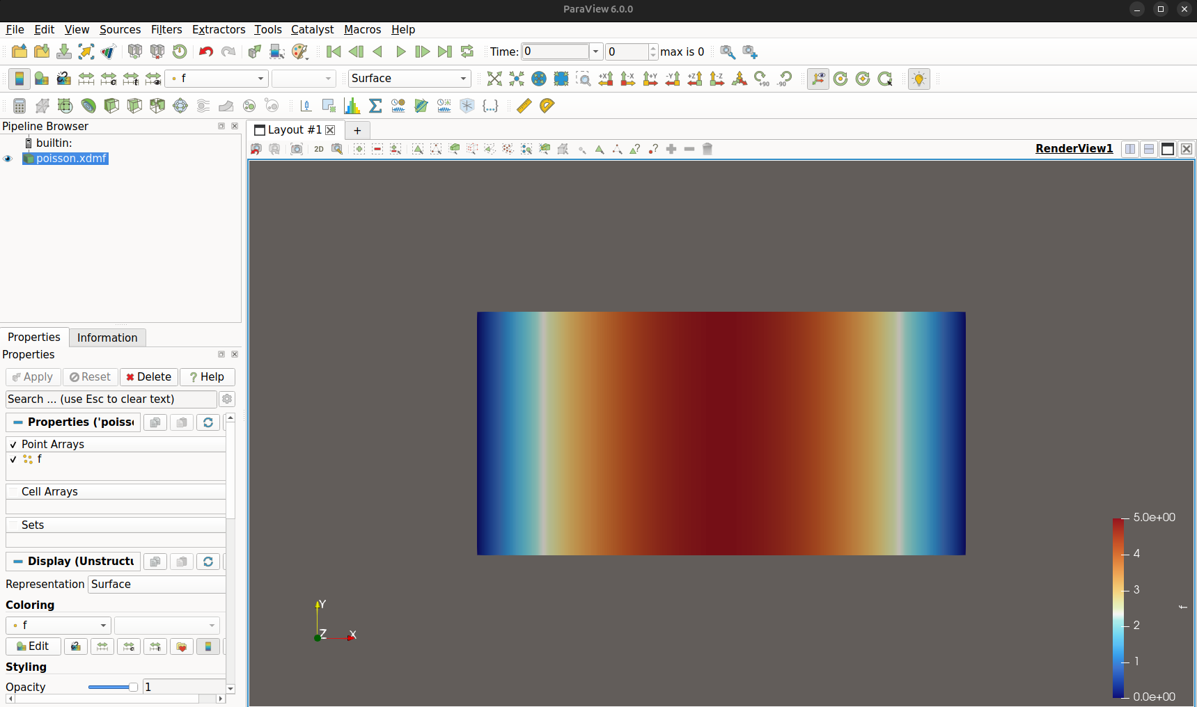
This solution visually corresponds to the analytical solution computed above ($u(x) = -5x^2 + 10x$).

Original tutorial’s version

The present subsection considers a more complex set of boundary conditions, as defined in the original tutorial:

• $g = \sin(5x)$
• $f = 10 \exp(-((x - 0.5)^2 + (y - 0.5)^2)/0.02)$

The input file demo_poisson_2.py defining this simulation is identical to the previous one except for the part that implements $g$ and $f$ functions’ expressions:

f = 10 * ufl.exp(-((x[0] - 0.5) ** 2 + (x[1] - 0.5) ** 2) / 0.02)
g = ufl.sin(5 * x[0])

The following command runs the simulation with this second set of boundary conditions:

apptainer exec fenics.sif python3 demo_poisson_2.py

As described above, the output file can be opened with Paraview as follows:

apptainer run paraview.sif out_poisson/poisson.xdmf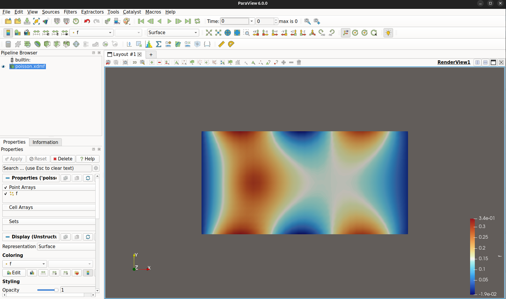

To go further

The official documentation provides multiple examples exhibiting the features of the software. Those examples can be easily run with the FEniCS container image by extrapolating the commands presented in this tutorial.